
Kelly Criterion: The Mathematics of Optimal Position Sizing
By Suyesh Gusain (B.Sc. Physics Hons., NISM Certified Research Analyst & Equity Derivatives)
Disclaimer: This article is strictly for educational and mathematical illustration purposes. It does not constitute financial, investment, or trading advice.
Imagine finding a biased coin that lands on heads 60% of the time, paying out 1:1 on your wager. You have a definitive, mathematically proven edge. You sit down with $1,000, feeling invincible.
How much do you wager on each flip?
If you bet $10 per flip, your capital grows at an agonizing crawl. If you bet $500 per flip, a mere sequence of two consecutive tails wipes out your bankroll entirely. This illustrates a foundational rule of probability: a positive mathematical edge alone does not protect you from total ruin.
The bridge between having an edge and compounding it safely is position sizing. In 1956, Bell Labs physicist John L. Kelly Jr. solved this challenge by formulating what is known today as the Kelly Criterion.
What Is the Kelly Criterion?
The Kelly Criterion is a mathematical formula used to determine the optimal size of a series of bets or investments to maximize long-term wealth growth.
John Kelly developed the concept while working alongside Claude Shannon—the father of information theory. Kelly was analyzing signal noise across long-distance telephone lines, addressing a core technical question: At what rate can data transmit across a noisy channel without distortion?
Kelly discovered that transmitting data through noise is mathematically identical to allocating capital under uncertainty. By treating portfolio growth as an information transmission problem, he introduced the Kelly Criterion to maximize the geometric growth rate of capital over time.
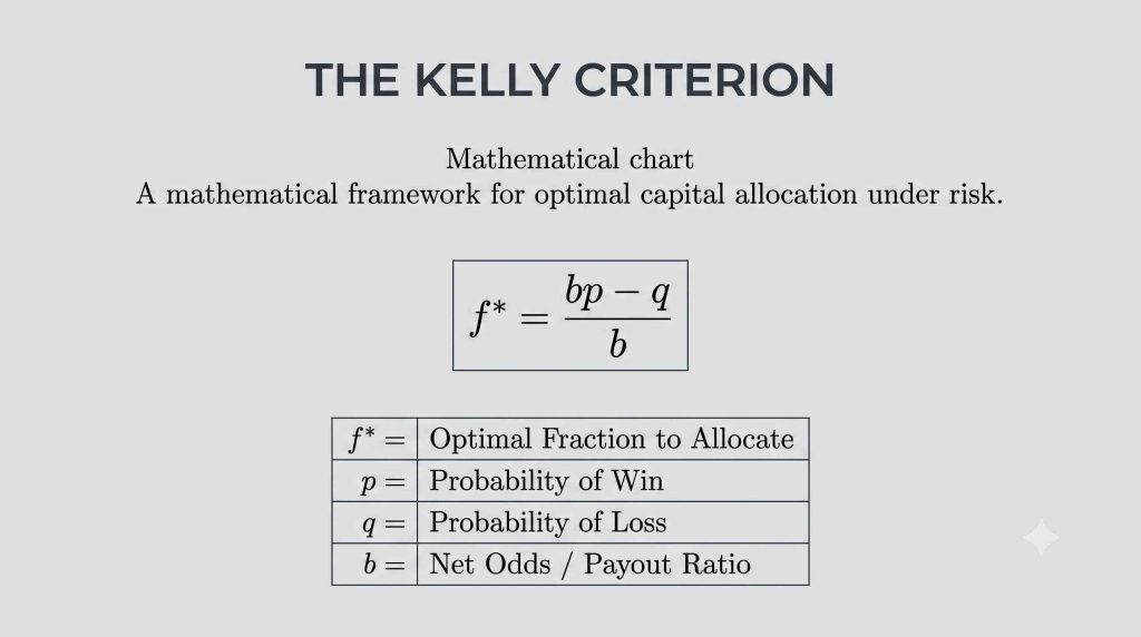
The Kelly Criterion Formula
The standard Kelly Criterion formula for binary outcomes is:
f* = (b × p − q) / b
Where:
- f* = The Kelly Criterion fraction of your current bankroll to allocate.
- b = The net decimal payout received on the wager (e.g., b = 1 for a 1:1 payout).
- p = The probability of winning.
- q = The probability of losing (1 − p).
Alternatively, the it can be expressed as:
Kelly Fraction = (Expected Net Profit) / (Payout Odds)
Worked Example: The 60% Coin
Applying the Kelly Criterion to a coin flip with a 60% win rate (p = 0.60) and an even 1:1 payout (b = 1):
- f* = [1(0.60) − 0.40] / 1 = 0.20 (or 20%)
It dictates allocating exactly 20% of your total capital to each flip:
- Allocating below the Kelly Criterion (< 20%): Compounding is suboptimal, leaving growth capacity underutilized.
- Allocating at the Kelly Criterion (= 20%): You achieve the maximum theoretical logarithmic compounding rate.
- Allocating above the Kelly Criterion (> 20%): Volatility drag rapidly degrades performance. At 40% (double Kelly), expected geometric growth drops to zero. Allocating beyond 40% ensures mathematical ruin over a sufficient sequence, despite the 60% edge.
Why the Kelly Criterion Focuses on Geometric Compounding
Standard arithmetic averages can be misleading. A +10% gain followed by a −10% loss results in a net 1% loss. In multiplicative systems:
- A 50% loss requires a 100% gain to break even.
- A 90% loss requires a 900% gain to recover.
The Kelly Criterion accounts for the asymmetry of losses by penalizing portfolio variance. Maximizing logarithmic wealth prevents deep drawdowns and keeps capital away from zero-absorbing barriers.
To explore how mathematical odds work in practice, read our deep dive into the roulette vs. blackjack house edge battle or learn how probability shapes payout mechanics in our guide on RTP and the house edge explained.
Full Kelly vs. Fractional Kelly in Real-World Markets
While the theoretical formula works cleanly on known coin flips, applying the Kelly Criterion to real financial markets introduces practical limitations:
| Risk Dimension | In Theory | In Practical Markets |
| Probability (p) | Static and known | Dynamic, non-stationary, and estimated |
| Payout Ratio (b) | Fixed binary payout | Variable, fat-tailed, subject to slippage |
| Drawdowns | Drawdowns exceeding 50% are normal | Psychologically and operationally unsustainable |
Because overestimating win rates or payout ratios moves an investor into negative compounding territory, market practitioners rarely use full Kelly Criterion sizing.
Instead, they apply Fractional Kelly:
- Half-Kelly (f* / 2): Captures roughly 75% of the maximum compounding rate while cutting portfolio variance and expected drawdowns by 50%.
- Quarter-Kelly (f* / 4): Sacrifices additional compounding speed to prioritize capital preservation and buffer against estimation errors.
End Note
A statistical edge only grants permission to enter the game; it is your allocation model that dictates whether you compound wealth or face inevitable ruin. The Kelly Criterion bridges this divide by solving for the mathematics of geometric compounding rather than deceptive arithmetic averages, penalizing excess volatility to prevent capital liquidation.
Because real financial markets are plagued by estimation errors, fat tails, and shifting regimes, dogmatic adherence to Full Kelly invites unsustainable drawdowns. By scaling back to Fractional Kelly, investors harness the formula’s core strength—maximizing long-term compounding—while securing an essential margin of safety against market uncertainty.
Author Bio
Suyesh Gusain is an analytical researcher and digital publisher specializing in algorithmic systems, data verification, and digital media ethics. Holding degrees in Physics (B.Sc. Hons) and Mass Communication (M.A.), Suyesh bridges the gap between rigorous mathematical analysis and accessible consumer education. His work centers on decoding complex algorithmic architectures, statistical probability, and digital integrity for modern audiences.
Please share your thoughts on this article in the comments below. If you found it helpful, make sure to share it with others and follow Wisdom Ganga on social media for more updates!
Frequently Asked Questions
What does the Kelly Criterion indicate if the result is negative?
If it yields a negative number or zero, your expected value is negative. In this situation, the optimal mathematical allocation is 0%, meaning the position should not be taken.
How does the Kelly Criterion compare to fixed-fractional sizing?
Fixed-fractional sizing allocates a static percentage (such as 1% per trade) regardless of edge. The Kelly Criterion dynamically adjusts allocation based on the specific probability and payout profile of each opportunity.
Can the Kelly Criterion lead to large drawdowns?
Yes. Full Kelly Criterion sizing is mathematically aggressive and can lead to drawdowns exceeding 50%. This is why quantitative traders and portfolio managers widely favor Fractional Kelly models to preserve a practical margin of safety.
How do you calculate the Kelly Criterion for stock trading?
To calculate the Kelly Criterion for stock trading, replace the fixed binary payout (b) with the ratio of your average winning trade to your average losing trade (Win/Loss Ratio, and set p as your historical win rate:
Kelly % = Win Rate − [(1 − Win Rate) / Win/Loss Ratio]
Because financial asset returns have fat tails, variable stop-outs, and regime shifts, traders routinely multiply the calculated Kelly percentage by 0.5 or 0.25 (Fractional Kelly) to avoid extreme portfolio drawdowns.
What is the difference between Kelly Criterion and Sharpe Ratio?
The Sharpe Ratio is a backward-looking performance metric that measures excess return per unit of total risk (standard deviation) to assess historical risk efficiency.
In contrast, the Kelly Criterion is a forward-looking sizing model designed to determine the precise capital percentage to allocate to maximize the geometric growth rate of wealth. While the Sharpe Ratio evaluates quality, the Kelly Criterion dictates execution size.
Why do Warren Buffett and Edward Thorp use the Kelly Criterion?
Legendary mathematician Edward Thorp first demonstrated the real-world application of the Kelly Criterion to beat blackjack and run early market-neutral quantitative hedge funds. Warren Buffett has similarly applied the underlying logic of the Kelly Criterion by taking aggressively sized, high-conviction positions when expected value significantly outstrips risk, while maintaining large cash buffers to avoid zero-absorbing ruin.
How does volatility drag affect the Kelly Criterion?
Volatility drag is the mathematical reduction in compound geometric return caused by dispersion in periodic returns. The Kelly Criterion solves directly for this friction: allocating beyond the optimal Kelly fraction amplifies volatility drag so severely that it turns a winning arithmetic edge into negative compound growth. Sizing at or below Kelly ensures that portfolio variance does not overwhelm capital compounding.